Compact Schemes for the Poisson Equation

8 minute read

If you prefer to follow in the notebook directly, you can also get the notebook.

Introduction

Finite differnce schemes can be derived from a taylor series expansion up to very large accuracy. The idea is to gain accuracy by increasing the number of points in the stencil. This works well, but can be cumbersome computationally as the stencils become very large and the modifications to the stencil that are required at the boundaries to maintain a uniform global accuracy are complex. This is where compact schemes become an interesting alternative.

Compact n$^{th}$-order derivative

Compact schemes are derived using a Taylor series expansion. Say we wish to construct a compact scheme with a three-point stencil using the value of the function at $x_{i-1}$, $x_i$ and $x_{i+1}$. If we used standard central difference schemes, this will only results in a 2$^{nd}$-order accurate approximation of $f'(x_i)$. In compact schemes, we not increase the order of accuracy by inclding neighbouring points of the unkown function derivative on the left-hand-side.

For the n$^{th}$ derivative we have the following system

\[L_{i-1}f^{(n)}_{i-1} + L_{i}f^{(n)}_{i} + L_{i+1}f^{(n)}_{i+1} = R_{i-1}f_{i-1} + R_{i}f_{i} + R_{i+1}f_{i+1},\]

where $L_j$ and $R_j$ are unkown coefficients. They are found by solving the linear system

\[\begin{bmatrix} \begin{matrix} 0 & 0 & 0 \end{matrix} & \begin{matrix} 1 & 1 & 1\\ \end{matrix}\\ Q^{(n)} & \begin{matrix} h_{i-1} & 0 & h_{i+1}\\ h_{i-1}^2/2! & 0 & h_{i+1}^2/2!\\ h_{i-1}^3/3! & 0 & h_{i+1}^3/3!\\ h_{i-1}^4/4! & 0 & h_{i+1}^4/4! \end{matrix}\\ \begin{matrix} 0 & 1 & 0 \end{matrix} & \begin{matrix} 0 & 0 & 0\\ \end{matrix}\\ \end{bmatrix}\begin{bmatrix} L_{i-1} \\ L_{i} \\ L_{i+1} \\ -R_{i-1} \\ -R_{i} \\ -R_{i+1}\\ \end{bmatrix}=\begin{bmatrix} 0\\ 0\\ 0\\ 0\\ 0\\ 1\\ \end{bmatrix},\]

where $h_{i-1}=x_{i-1}-x_i$ and $h_{i+1} = x_{i+1}-x_i$. The sub-matrix $Q^{(n)}$ depends on the derivative required. For the first derivative, we have

\[Q^{(1)} = \begin{bmatrix} 1 & 1 & 1\\ h_{i-1} & 0 & h_{i+1}\\ h_{i-1}^2/2! & 0 & h_{i+1}^2/2!\\ h_{i-1}^3/3! & 0 & h_{i+1}^3/3!\\ \end{bmatrix}\]

and for the second derivative

\[Q^{(2)} = \begin{bmatrix} 0 & 0 & 0\\ 1 & 1 & 1\\ h_{i-1} & 0 & h_{i+1}\\ h_{i-1}^2/2! & 0 & h_{i+1}^2/2!\\ \end{bmatrix}.\]

def get_compact_coeffs(n, hi):
    # assumes uniform grid
    h_i = -hi
    r = np.hstack((np.array([0 for i in range(5)]),1.))
    L = np.array([[0, 0, 0, 1, 1, 1],
                  [0, 0, 0, h_i, 0, hi],
                  [0, 0, 0, h_i**2/fact(2), 0, hi**2/fact(2)],
                  [0, 0, 0, h_i**3/fact(3), 0, hi**3/fact(3)],
                  [0, 0, 0, h_i**4/fact(4), 0, hi**4/fact(4)],
                  [0, 1, 0, 0, 0, 0]])
    insert = np.array([[1,           1,                1],
                       [h_i,         0,               hi],
                       [h_i**2/fact(2), 0, hi**2/fact(2)],
                       [h_i**3/fact(3), 0, hi**3/fact(3)]])
    L[n:5,:3] = insert[:-n+5,:]
    vec = np.round(np.linalg.solve(L, r), 8)
    return vec[:3], -vec[3:]

We can check that for a first derivative, we recover the standard Pade ($4^{th}$-order) coefficients, which are

\[L = \left[\frac{1}{4}, 1, \frac{1}{4}\right], \qquad R = \left[-\frac{3}{4}, 0., \frac{3}{4}\right]\]

pade = np.array([1./4., 1., 1./4., -3./4., 0., 3./4.])
np.allclose(np.hstack(get_compact_coeffs(1, 1)), pade)

True

We can now write a function that, given a function $f$, on a uniform grid with spacing $dx$, return the $n^{th}$ derivative of that function. Because for each point we solve for the compact coefficients, we can in theory get compact schemes on non-uniform grid with the same accuracy. Here we will only focus on uniform grids.

def derive_compact(n, f, dx):
    
    # get coeffs
    L, R = get_compact_coeffs(n, dx)
    
    # temp array
    sol = np.empty_like(f)
    
    # compact scheme on interior points
    sol[2:-2] = R[0]*f[1:-3] + R[1]*f[2:-2] + R[2]*f[3:-1]
    
    # boundary points
    sol[-2] = R[0]*f[-3] + R[1]*f[-2] + R[2]*f[-1]
    sol[-1] = R[0]*f[-2] + R[1]*f[-1] + R[2]*f[-0]
    sol[ 0] = R[0]*f[-1] + R[1]*f[ 0] + R[2]*f[ 1]
    sol[ 1] = R[0]*f[ 0] + R[1]*f[ 1] + R[2]*f[ 2]
    
    # build ugly matrix by hand
    A = sparse.diags(L,[-1,0,1],shape=(len(f),len(f))).toarray()
    # periodic BS's
    A[ 0,-1] = L[0]
    A[-1, 0] = L[2]
        
    return np.linalg.solve(A, sol)

We can then test the method on a known function, with known first and second derivaive. For simplicity, we will use trigonometric functions, which have an infinite number of well-behaved derivatives

\[f(x) = \sin(x), \,\, x\in[0, 2\pi).\]

With

\[\frac{d}{dx}f(x) = \cos(x), \quad \frac{d^2}{dx^2}f(x) = -\sin(x), \,\, x\in[0, 2\pi).\]

N = 128
x, dx = np.linspace(0, 2*np.pi, N, retstep=True, endpoint=False)
function = np.sin(x)

# first derivative
sol = derive_compact(1, function, dx)
print('First derivative L2 norm:  ', norm(sol-np.cos(x)))

# second derivative
sol = derive_compact(2, function, dx)
print('Second derivative L2 norm: ', norm(sol+np.sin(x)))

First derivative L2 norm:   2.00356231982653e-09
Second derivative L2 norm:  1.5119843767976088e-09

Poisson Equation With Compact Schemes

We aim to solve the following one-dimensionnal Poisson equation with Dirichlet boundary conditions

\[\begin{split} -&\frac{d^2}{dx^2}u(x) = f(x), \quad a<x<b\\ &u(a) = 0, \quad u(b) = 0\\ \end{split}\]

where $a, b\in\mathbb{R}$, $u(x)$ is the unkown function and $f(x)$ is some given source term.

The approach that we will use here is different, in this case, we know the value of the derivatie of the function $u$, they are equal to the source term. We want to re-write our Poisson equation in terms of the unkown function $u$ (and not it’s derivative $u'$) as a function of $f$. To do so, we discretize the left side of the Poisson equation ($u''_i$) using a compact finite difference scheme with fourth-order accuracy on a uniform grid with grid points located at $x_i = a+ih,$ $ h=(b-a)/M,$ with $i=0, 1, 2,…, M$ where $M$ is a positive integer, as we would if the derivatives where the unknown. This gives

\[\frac{1}{10}u''_{i-1} + u''_i + \frac{1}{10}u''_{i+1} = \frac{6}{5}\frac{u_{i+1} + 2u_i + u_{i-1}}{h^2},\]

or in a more common form,

\[u''_{i-1} + 10u''_i + u''_{i+1} = \frac{12}{h^2}\left(u_{i+1} + 2u_i + u_{i-1}\right).\]

Because we are using points $\pm1$ away from $x_i$, this results in a tri-diagonal system

\[AU''= \frac{12}{h^2}BU,\]

where $U'' = (u''_1,u''_2,...,u''_M)^\top$ and $U = (u_1,u_2,...,u_M)^\top\in \mathbb{R}^{M-1}$. The tri-diagonal matrix $A, B \in \mathbb{R}^{M-1\times M-1}$ are

\[A = \begin{bmatrix} 10 & 1 & 0 &\dots & 0 & 0 \\ 1 & 10 & 1 &\dots & 0 & 0 \\ 0 & 1 & 10 &\dots & 0 & 0 \\ \vdots & \vdots & \vdots & \ddots & \vdots & \vdots \\ 0 & 0 & 0 & \dots & 10 & 1 \\ 0 & 0 & 0 &\dots & 1 & 10 \\ \end{bmatrix}, \qquad B = \begin{bmatrix} -2 & 1 & 0 &\dots & 0 & 0 \\ 1 & -2 & 1 &\dots & 0 & 0 \\ 0 & 1 & -2 &\dots & 0 & 0 \\ \vdots & \vdots & \vdots & \ddots & \vdots & \vdots \\ 0 & 0 & 0 & \dots & -2 & 1 \\ 0 & 0 & 0 &\dots & 1 & -2 \\ \end{bmatrix}.\]

To find the unkwon values of $U$, we just need to invert the system, but $U''$ is still unkown! Well actually, it is know from the Poisson problem $-u''(x_i)=f(x_i), i=1,2,...,M-1$ i.e. $-U''=F$. Substituting this result in the previous linear system gives

\[-\frac{12}{h^2}BU = AF,\]

def build_AB(M, h):
    A = sparse.diags([1.,10.,1.],[-1,0,1],shape=(M, M)).toarray()
    B = sparse.diags([1.,-2.,1.],[-1,0,1],shape=(M, M)).toarray()
    # dont forget BC, here homogeneous Dirichlet
    B[ 0,:]=0.; B[ 0, 0]=1
    B[-1,:]=0.; B[-1,-1]=1
    return A, -12./h**2*B

To obtaine the solution $U$, we simply need to solve it! The $B$ matrix is symmetric and positively-definite, it is trivial to solve.

def SolvePoissonCompact(f, h, M):
    u0 = np.zeros_like(f)
    A, B = build_AB(M, h)
    sigma = np.matmul(A, f)
    return np.linalg.solve(B, sigma)

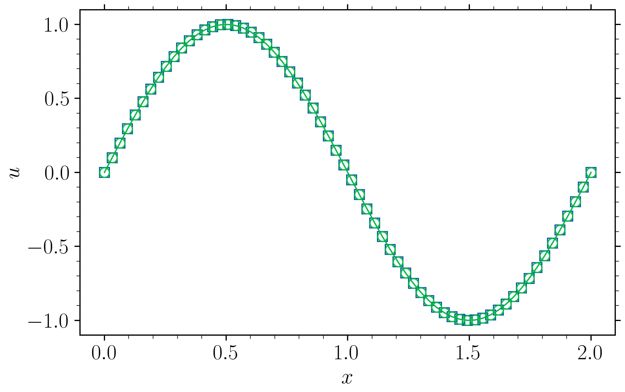
Example 1.

In the first example, we consider the problem with homogeneous Dirichlet boundary conditions

\[\begin{cases} -u''(x) = \pi^2\sin(\pi x), & 0 < x <2,\\ u(0)=0, \quad u(2) = 0. \end{cases}\]

The exact solution is $u_e(x)=\sin(\pi x)$.

M = 64
x, h = np.linspace(0., 2., M, retstep=True, endpoint=True)
f = np.pi**2*np.sin(np.pi*x)
u_e = np.sin(np.pi*x)
u_num =  SolvePoissonCompact(f, h, M)
print(norm(u_num-u_e))
plt.plot(x, u_e, '-s')
plt.plot(x, u_num,'-o')

which gives you

6.02248257496857e-06

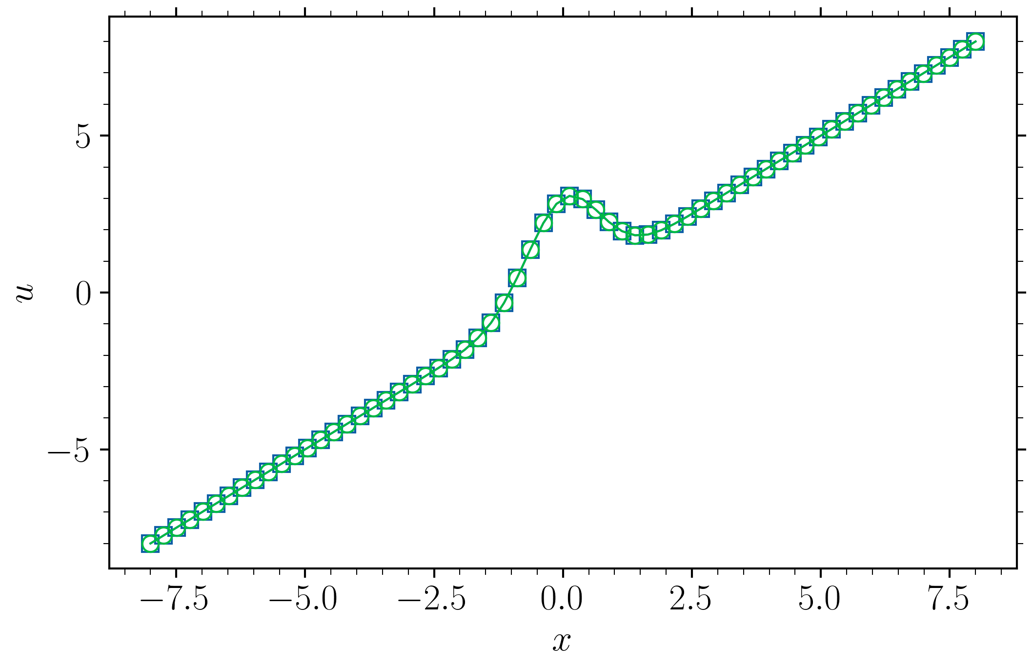
Example 2.

Now with non-zero Dirichlet Boundry conditions

\[\begin{cases} -u''(x) = 12e^{-x^2}(-x^2+1/2), & -8 < x <8,\\ u(-8)=-8, \quad u(8) = 8. \end{cases}\]

The exact solution is $u_e(x)=3e^{-x^2}$. In the numerical computation, we make use of a change of variable $U(x)=u(x)-x$ to solve this problem. Applying the numerical algorithm, we now have

\[\begin{cases} -U''(x) = 12e^{-x^2}(-x^2+1/2), & -8 < x <8,\\ U(-8)=-0, \quad U(8) = 0. \end{cases}\]

and the approximate numerical solution at a grid point is found as $u(x) = U(x)=x$.

    M = 64
    x, h = np.linspace(-8., 8., M, retstep=True, endpoint=True)
    f = 12.*np.exp(-x**2)*(-x**2 + 0.5)
    u_e = 3.*np.exp(-x**2)+x
    u_num = SolvePoissonCompact(f, h, M)
    print(norm(u_num-u_e))
    plt.plot(x, u_e, '-s')
    plt.plot(x, u_num+x,'-o')

0.5864429590964948

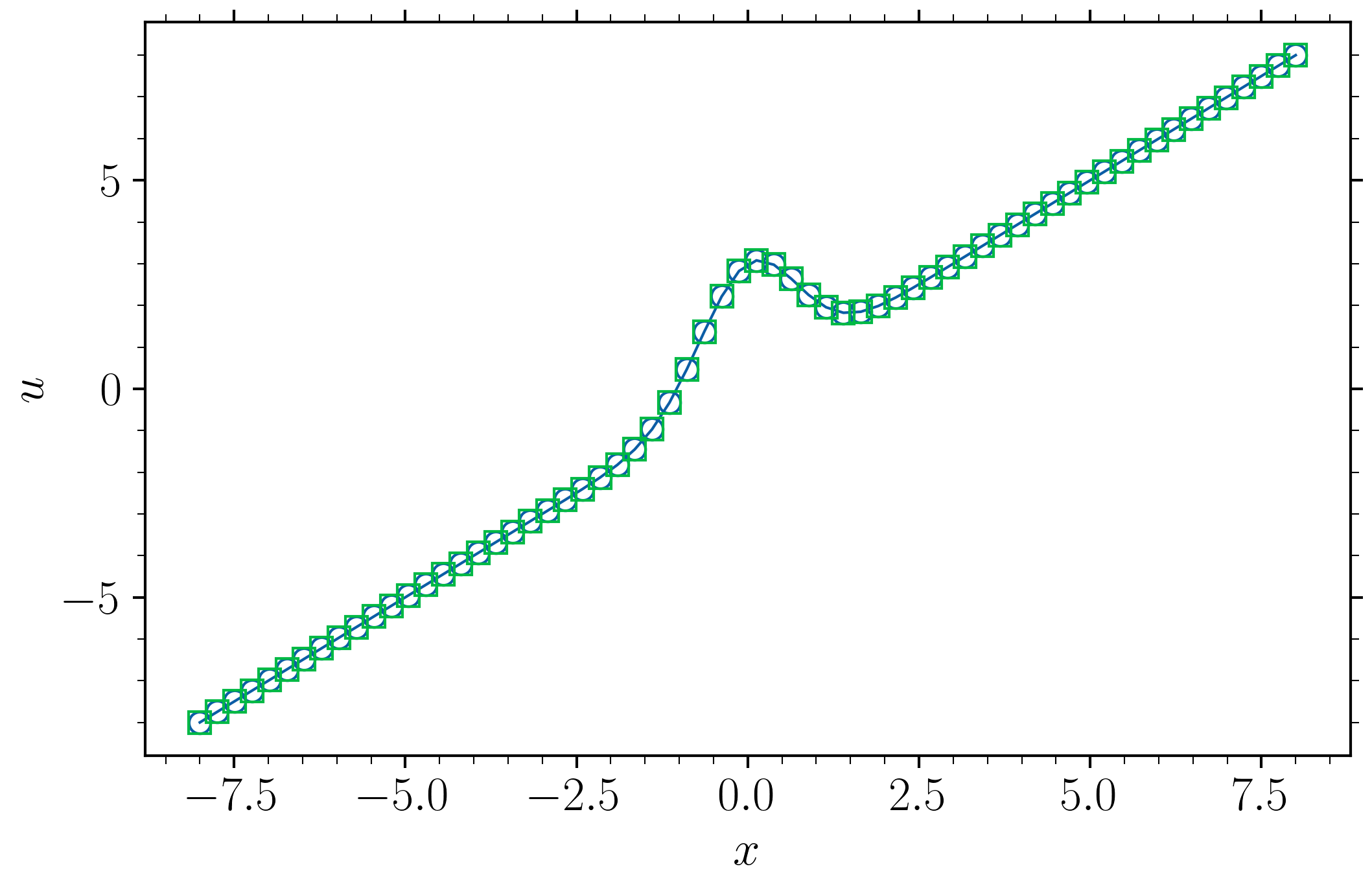
Using Faste Fourier Transforms to Solve the Poisson Equation

We actually do not need ton inverte the system described earlier to get the solution, see. We can use the Sine transform for $U\in\mathbb{R}^{M-1}$

\[\begin{split} u_j &= \sum_{k=1}^{M-1}\hat{u}_k\sin\left(\frac{jk\pi}{M}\right), \,\, j=1,2,...,M-1,\\ \hat{u_k} &= \frac{2}{M}\sum_{j=1}^{M-1}u_j\sin\left(\frac{ik\pi}{M}\right), \,\, j=1,2,...,M-1, \end{split}\]

from whcih we can approximate $u_{i+1}$, $u_{i-1}$, $u''_{i+1}$, $u''_{i-1}$ as

\[\begin{align} u_{i+1}=\sum_{k=1}^{M-1}\hat{u}_k\sin\left(\frac{(i+1)k\pi}{M}\right),\qquad & u_{i-1} = \sum_{k=1}^{M-1}\hat{u}_k\sin\left(\frac{(i-1)k\pi}{M}\right)\\ u''_{i} =\sum_{k=1}^{M-1}\hat{u}''_k\sin\left(\frac{ik\pi}{M}\right),\qquad & u''_{i+1} =\sum_{k=1}^{M-1}\hat{u}''_k\sin\left(\frac{(i+1)k\pi}{M}\right)\\ u''_{i-1} =\sum_{k=1}^{M-1}\hat{u}''_k\sin\left(\frac{(i-1)k\pi}{M}\right). & \\ \end{align}\]

Subsituting in the compact discretization of the Poisson equation gives,

\[\begin{split} \sum_{k=1}^{M-1}\hat{u}''_k\left\{ \frac{1}{10}\sin\left(\frac{(i-1)k\pi}{M}\right) + \sin\left(\frac{ik\pi}{M}\right) + \frac{1}{10}\sin\left(\frac{(i+1)k\pi}{M}\right) \right\} =\\ \frac{6}{5h^2}\sum_{k=1}^{M-1}\hat{u}_k\left\{ \sin\left(\frac{(i-1)k\pi}{M}\right) +\sin\left(\frac{(i+1)k\pi}{M}\right) - 2\sin\left(\frac{ik\pi}{M}\right) \right\} \end{split}\]

or, after rearranging

\[\hat{u}_k = -\hat{u}''_k\left(\frac{24\sin^2\left(\frac{k\pi}{2M}\right)}{h^2}\right)^{-1}\left(\cos\left(\frac{k\pi}{M}\right)+5\right), \,\, k\in 1,2,..,M-1.\]

In addition, we obtain $-u''_{i} = f_i \,(i=1,2,...,M-1)$. By the inverse Sine transform, we get to know $-\hat{u}''_k=\hat{f}_k \, (k=1,2,...,M-1)$, which allows us to solve for $\hat{u}$

\[\hat{u}_k = \hat{f}_k\left(\frac{24\sin^2\left(\frac{k\pi}{2M}\right)}{h^2}\right)^{-1}\left(\cos\left(\frac{k\pi}{M}\right)+5\right), \,\, k\in 1,2,..,M-1.\]

Note: We use a spectral method to solve the tri-diagonal system, this doesn’t mean we solve it with spectral accuracy, here the modified wavenumber makes the spectral method the exact same accuracy as the compact scheme.

def SolvePoissonSine(f, h, M):
    f_k = fftpack.dst(f, norm='ortho')
    k = np.arange(1,M+1)
    u_k = f_k*(24*np.sin(k*np.pi/(2*M))**2./h**2.)**(-1.)*(np.cos(np.pi*k/M)+5.)
    return fftpack.idst(u_k, norm='ortho')

M = 64
x, h = np.linspace(-8, 8, M, retstep=True, endpoint=True)
f = 12.*np.exp(-x**2)*(-x**2 + 0.5)
u_e = 3.*np.exp(-x**2)+x
u_num = SolvePoissonSine(f, h, M)
print(norm(u_num-u_e))
plt.plot(x, u_num + x, '-o')
plt.plot(x, u_e, 's');

0.5864429590964948

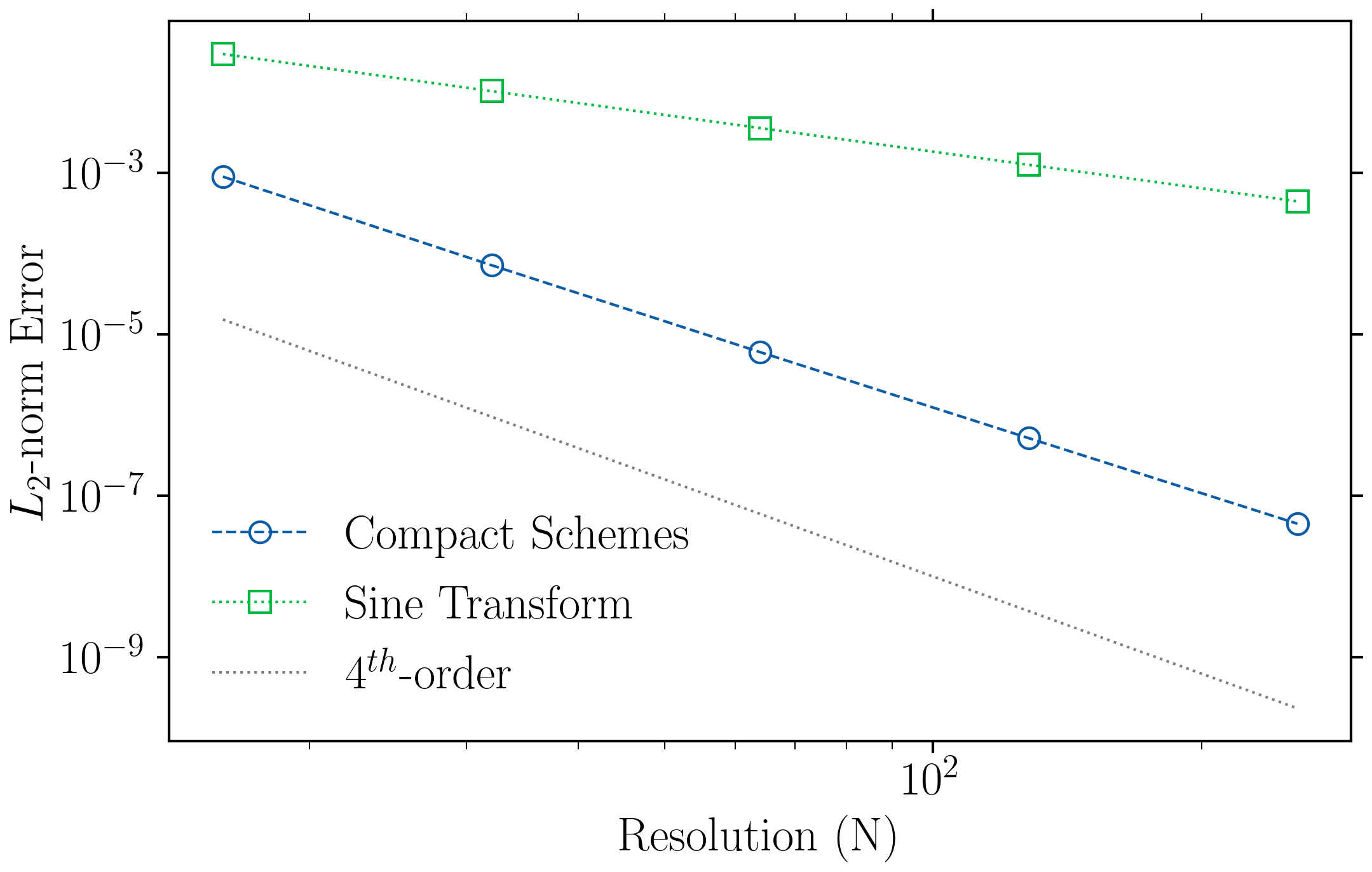
Order of Accuracy

L2_com = []
L2_Sine = []
Resolutions = 2.**np.arange(4,9)
for N in Resolutions:
    x, h = np.linspace(0., 2., int(N), retstep=True, endpoint=True)
    f = np.pi**2*np.sin(np.pi*x)
    u_e = np.sin(np.pi*x)
    u_num = SolvePoissonCompact(f, h, int(N))
    error = norm(u_num-u_e)
    L2_com.append(error)
    u_num = SolvePoissonSine(f, h, int(N))
    error = norm(u_num-u_e)
    L2_Sine.append(error)
plt.loglog(Resolutions, np.array(L2_com), '--o', label='Compact Schemes')
plt.loglog(Resolutions, np.array(L2_Sine), ':s', label='Sine Transform')
plt.loglog(Resolutions, Resolutions**(-4), ':k', alpha=0.5, label=r"$4^{th}$-order")
plt.xlabel("Resolution (N)"); plt.ylabel(r"$L_2$-norm Error")
plt.legend()

2023

Topographic map of Switzerland

3 minute read

Installing custom colormap in windy.com

2 minute read

2021

Lagrangian Coherent Structures: Finite-Time Lyapunov Exponent

7 minute read

Advanced Scientific Matplotlib - Part 1/n