Lagrangian Coherent Structures: Finite-Time Lyapunov Exponent

6 minute read

Introduction

In the study of dynamical systems, Lagrangian Coherent Structures (LCS) are an essential tool to distinguish material surface formed by trajectories that exert a consistent action on nearby trajectories. A classical example of an attracting material surface in dynamical system is called an attractor, see the Lorenz System for example.

One big advantage of using LCS (or in other words tracking particles trajectories) to analyse dynamical systems is their Galilean invariance, unlike Eulerian criteria.

A common way of determining these LCS is trough ridges of the Finite-time Lyapunov (FTLE). In the following, I will detail how this ridges are computed based on numerical results of a simple flow field.

Double-Gyre flow

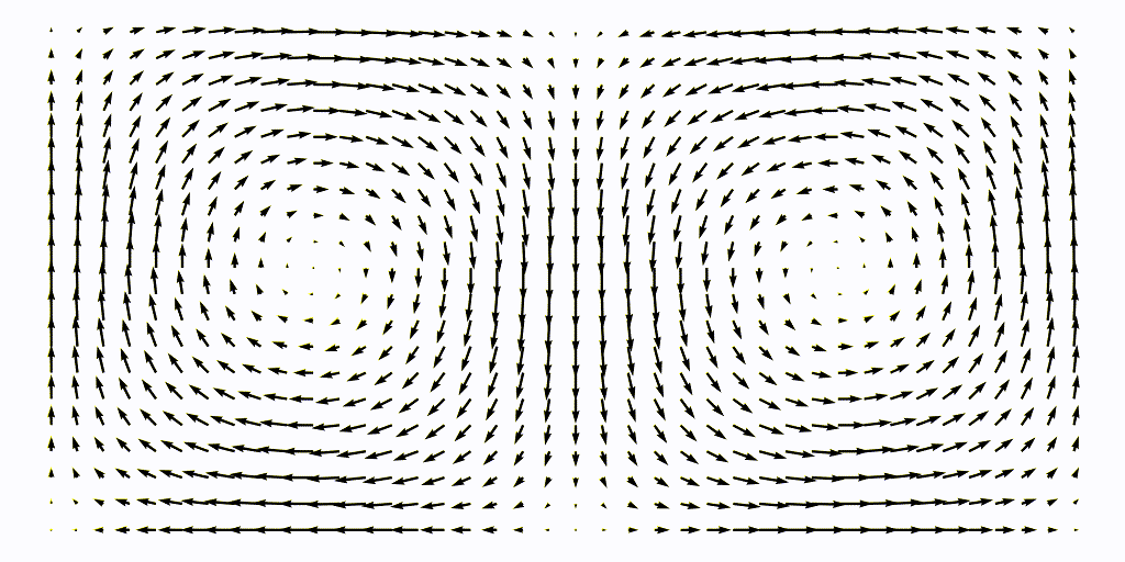
The periodically varying double-gyre flow was discussed in Shadden et al. (2005). It is used as a standard test case for LCS and can be considered a local view of a gulf stream ocean front. It is described by the stream-function

\[\psi(x, y, t) = A\sin(\pi f(x, t)) \sin(\pi y)\]

where

\[f(x, t) = \epsilon\sin(\omega t)x^2 + (1-2\epsilon\sin(\omega t))x,\]

the two component of the time-varying velocity field are then found with the definition of the stream-function $\psi = \nabla\times u$ which gives for a 2D case

\[u = -\frac{\partial \psi}{\partial y}, \qquad v = \frac{\partial \psi}{\partial y}.\]

The flow is defined over a domain $L\times H = [0, 2] \times [0, 1]$, see the animation below

double_gyre

Computation of the FTLE

To compute FTLE we start with a standard time-dependent velocity field $\vec u \in \mathbb{R}^n \times T$ and a particle trajectory that satisfies

\[\dot{\vec x}(t) = \vec u(\vec x(t), t).\]

In the following example an analytical solution for the time-dependent velocity field $\vec u$ is provided, but it is much more common that this velocity field is obtained from discrete (in time and space) results of numerical simulations, one must therefore use interpolation to find the value of the velocity field between those points.

To compute the FTLE, the approach is to seed the flow with passive particles with location $X_0 \subset \mathbb{R}^n$. The particle’s trajectories are then advected/intergated forward (or backward) in time from the initial time $t-0$ to the final time $t=T$ to obtain the time-T flow-map defined as

\[\Phi_0^T : \mathbb{R}^n \to \mathbb{R}^n; \quad \vec{x}(0) \to \vec x (0) + \int_{0}^{T} \vec u(\vec x(\tau), \tau)\text{ d}\tau.\]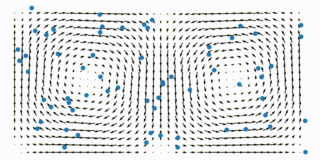

double_gyre_p

Once the flow map is obtained, we can compute the deformation gradient tensor ${\bf D}\Phi_0^T$ of every particle, usually by finite-difference (using the 2D deformation gradient as an example)

\[{\bf D}\Phi_0^T = \begin{bmatrix} \frac{\partial X}{\partial x} & \frac{\partial X}{\partial y} \\ \frac{\partial Y}{\partial x} & \frac{\partial Y}{\partial y} \\ \end{bmatrix} \sim \begin{bmatrix} \frac{X_{i+1,j}(T) - X_{i-1,j}(T)}{x_{i+1,j}(0) - x_{i-1,j}(0)} & \frac{X_{i+1,j}(T) - X_{i-1,j}(T)}{y_{i+1,j}(0) - y_{i-1,j}(0)} \\ \frac{Y_{i+1,j}(T) - Y_{i-1,j}(T)}{x_{i+1,j}(0) - x_{i-1,j}(0)} & \frac{Y_{i+1,j}(T) - Y_{i-1,j}(T)}{x_{i+1,j}(0) - x_{i-1,j}(0)} \\ \end{bmatrix},\]

where $X$ and $x$ are understood to be Lagrangian and Eulerian variables. The finite-difference approximation assumes that we started with a uniform particles distribution. The deformation grandient measures the amount of stretching a particule experienced during the time interval $T$. Next, the Cauchy-Green deformation tensor can be computed

\[{\bf C}_0^T = ({\bf D}\Phi_0^T)^\top{\bf D}\Phi_0^T,\]

where $(.)^\top$ denote the transpose operator. The maximum amount of stretching experienced by the particle is obtained from maximum eigenvalue $\lambda_{\text{max}}$ of the Cauchy-Green deformation tensor. This is equivalent to performing a singular-value decomposition of this tensor. This is then synthesized into a FTLE field for the time-T flow map

\[\sigma(\Phi_0^T; \vec x_0) = \frac{1}{|T|}\log\sqrt{\lambda_{\text{max}}({\bf C}_0^T(\vec x_0))}\]

Note: This is the procedure to obtain the FTLE of the time-T flow map, this means that these ridges represent attracting/repeling LCS for particles with initial position $t=0$, for a time-varying velociy field, the FTLE field is obtained by numerous integration of these trajectories with the initial condition varying every time, this can be very expansive!

Numerical Implementation in `Julia`

First, we start by importing the required libraries, here we need the LinearAlgebra and PyPlot libraries, off course you can also use another ploting library if you prefer

using LinearAlgebra
using PyPlot

Next we need to define the function f, the time-varying part of our flow model

\[f(x, t) = \epsilon\sin(\omega t)x^2 + (1-2\epsilon\sin(\omega t))x,\]

which, once transalated to the Julia language gives

function f(x, t, omega, epsilon)
    return epsilon*sin(omega*t)*x^2 + (1-2*epsilon*sin(omega*t))*x.
end

We can then define our stream-function based on this function

function phi(x, y, t, A=0.1, omega=2pi/10, epsilon=0.2)
    return @. A*sin(pi*f(x, t, omega, epsilon)) * sin(pi*y)
end

Note: Note here that we must broadcast the results with @.

As we will generate a mesh of particle and advect it, we must be able to compute the local flow velocity at any point in space and in time, luckily we do not need to interpolate here, we can just compute the value of the velocity at a given location $\vec r = [x, y]$ using the gradient of the stream-function

function update(r, t, Delta=0.0001)
    x = r[:,1]; y = r[:,2]
    vx = (phi(x,y.+Delta,t).-phi(x,y.-Delta,t))./(2*Delta)
    vy = (phi(x.-Delta,y,t).-phi(x.+Delta,y,t))./(2*Delta)
    return [-vx -vy]
end

Where we have used a standard central difference to esimate the gradient of the stream-function.

Once we have our particle position at time $T$ (I will detail later how to achieve this) we need to compute the local Cauchy-Green deformation tensor. This could be a complex task, but because we will start with a uniform distribution of particles, neighbouring particles are located at neighbouring indices, which makes things much simpler!

function Jacobian(x, y, delta)
    
    # pre-processing
    nx, ny = size(x)
    J = Array{Float64}(undef, 2, 2)
    FTLE = Array{Float64}(undef, nx-2, ny-2)

    for j ∈ 1:ny-2, i ∈ 1:nx-2
        
        # jacobian of that particle
        J[1,1] = (x[i+2,j]-x[i,j])/(2*delta)
        J[1,2] = (x[i,j+2]-x[i,j])/(2*delta)
        J[2,1] = (y[i+2,j]-y[i,j])/(2*delta)
        J[2,2] = (y[i,j+2]-y[i,j])/(2*delta)

        # Green-Cauchy tensor
        D = transpose(J).*J
        
        # its largest eigenvalue
        lamda = eigvals(D)
        FTLE[i,j] = maximum(lamda)
    end
    return FTLE
end

Alright, now we can start to look at advecting the particle to find their final position. We will use a $4^{th}$-order Runge-Kutta method to integrate the equation

\[\dot{\vec x}(t) = \vec u(\vec x(t), t) \sim f(\vec x(t), t)\]

from time $t_n$ to $t_{n+1} = t_n + \Delta t$ following

\[\begin{split} k_1 &= \Delta t \, f(\vec r_n, t_n)\\ k_2 &= \Delta t \, f(\vec r_n + 0.5k_1, t_n+0.5\Delta t)\\ k_3 &= \Delta t \, f(\vec r_n + 0.5k_2, t_n+0.5\Delta t)\\ k_4 &= \Delta t \, f(\vec r_n + k_3, t_n+\Delta t)\\ \vec{r}_{n+1} &= (k_1 + 2k_2 + 2k_3 + k_4 ) / 6. \end{split}\]

We also need to define a grid of particles to advect. Because the edges of the domain have zero velocity, the particles there won’t move so we won’t bother putting particles on the boundary itself

# number of positions
N = 256

# particle position (2D grid)
x = collect(LinRange(0.01, 1.99, 2*N))' .* ones(N)
y = collect(LinRange(0.01, 0.99,   N))  .* ones(2*N)';

# particle positions
r = [vec(x) vec(y)]

Then we can proceed to intergate in time to find the first flow map $\Phi_{0}^{T}$

# time step
dt = 0.1
T = collect(range(0, 20, step=dt))

# intergate in time with RK4
for t ∈ T
    k1 = dt*update(r, t)
    k2 = dt*update(r+0.5*k1, t+0.5*dt)
    k3 = dt*update(r+0.5*k2, t+0.5*dt)
    k4 = dt*update(r+k3, t+dt)
    r += (k1 + 2*k2 + 2*k3 + k4) / 6
end

The resulting advection of a uniform aprticle grid is shown below, the particles are colored with the instantaneous FTLE values

flow_map

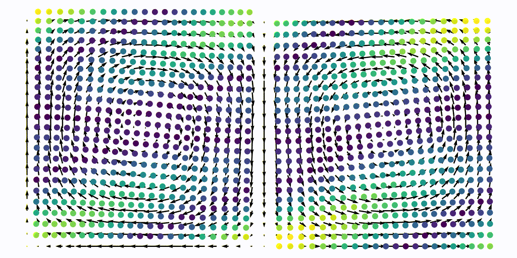
Once we have integrated this flow map, we can extract the $x$ and $y$ coordinates of each points and compute the FTLE using our Jacobian function

# extract position
x = reshape(r[:,1], N, 2*N);
y = reshape(r[:,2], N, 2*N);

# compute FTLE
FTLE = Jacobian(x, y, r[1,2]-r[1,1])
FTLE = log.(FTLE);

We can the proceed to plot the results

contour(FTLE, levels=31, cmap="viridis")

Because the flow is time-dependent, we must perform this integartion for every time-step. This means re-generating the array of particle, but now at time $t=\Delta t$, such that we now obtain the flow map $\Phi_{\Delta t}^{T+\Delta t}$, and so on.

Once this is done we can assemble the time-varying FTLE field of the double-gyre flow

FTLE_double_gyre

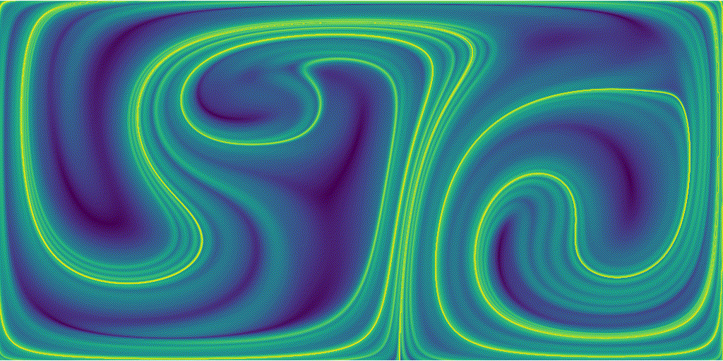
Areas of high sretching are represented by the sharp green ridges, particules that started at this location experienced a larger stretching than particles that started from bluer regions.

We can notice that because the base flow is periodic, our FTLE field is also periodic.

Inspiration

Steve Brunton’s brillant video!

2023

Topographic map of Switzerland

3 minute read

Installing custom colormap in windy.com

2 minute read

2021